
Rate of Return: Historical Insights for Smart Investors
Understanding investment performance requires mastering one of the most fundamental concepts in finance: the rate of return. This metric serves as the cornerstone for evaluating whether an investment has generated profits or losses over a specific period. For investors, students, and financial professionals analyzing historical market movements, comprehending how returns are calculated and interpreted provides essential context for spotting patterns and learning from past market behavior. By examining the rate of return concept across different assets and time periods, we can better understand the stories behind significant market events and make more informed decisions going forward.
What Rate of Return Measures in Financial Markets
The rate of return represents the percentage change in an investment's value over a defined time period. This metric captures both income received (such as dividends or interest) and capital appreciation (or depreciation) in a single, comparable figure.
When examining historical market data, the rate of return allows investors to standardize performance across different asset types, investment sizes, and timeframes. A $1,000 investment that grows to $1,200 delivers the same 20% return as a $100,000 investment that reaches $120,000, making comparisons meaningful regardless of scale.
Core Components of Return Calculation
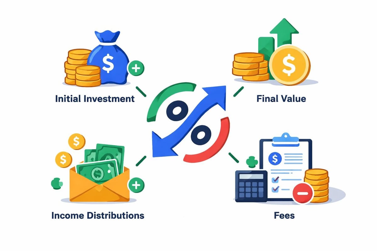
Every return calculation incorporates several key elements that together determine overall performance:
- Initial investment value at the beginning of the measurement period
- Ending investment value at the conclusion of the period
- Income distributions received during the holding period
- Time horizon over which the investment was held
- Costs and fees that reduce net returns
The basic formula expresses the rate of return as a percentage of the original investment. Specifically, you subtract the initial value from the final value, add any income received, divide by the initial value, and multiply by 100 to convert to a percentage.
Historical Perspectives on Investment Returns
Analyzing historical returns reveals patterns that help investors understand market behavior across different economic conditions. The stock market's long-term average annual return of approximately 10% before inflation masks tremendous variation across different periods and sectors.
During the Roaring Twenties, investors experienced extraordinary returns before the devastating losses of the 1929 crash and subsequent Great Depression. These dramatic swings in the rate of return illustrate how economic cycles, policy decisions, and market sentiment interact to drive performance.
Comparing Asset Classes Through Time
Different asset classes have delivered varying rates of return throughout financial history. Examining these differences provides crucial context for portfolio construction and risk management.
| Asset Class | Average Annual Return (1926-2025) | Volatility Level | Notable Historical Periods |
|---|---|---|---|
| Large-Cap Stocks | 10.2% | High | Great Depression, Dot-com Bubble |
| Small-Cap Stocks | 12.1% | Very High | 1975-1983 Surge, 2008 Crisis |
| Corporate Bonds | 6.3% | Moderate | 1980s Rate Decline |
| Government Bonds | 5.5% | Low | Post-WWII Period |
| Treasury Bills | 3.3% | Very Low | Inflation Hedge 1970s |
Understanding these historical benchmarks helps investors set realistic expectations and evaluate whether specific investments have outperformed or underperformed their asset class averages.
Calculation Methods for Different Investment Types
The approach to calculating the rate of return varies depending on the investment vehicle and the complexity of cash flows involved. Simple investments with a single purchase and sale point use straightforward calculations, while investments with multiple contributions or withdrawals require more sophisticated methods.
Simple Rate of Return
For basic investments without interim cash flows, the calculation remains relatively straightforward. An investor who purchased shares at $50 and sold them at $65 while receiving $3 in dividends achieved a return of 36%: ($65 - $50 + $3) / $50 = 0.36 or 36%.
This method works well for analyzing historical trades or investment positions held for specific periods without additional contributions. Historical market analysis often employs this approach when examining how individual stocks or assets performed during notable market events.
Annualized Rate of Return
Comparing investments held for different durations requires annualizing returns to create an apples-to-apples comparison. A 50% return over five years differs significantly from a 50% return over one year, even though the absolute percentage appears identical.
The annualized return formula accounts for compounding over multiple periods:
Annualized Return = [(Ending Value / Beginning Value)^(1/Number of Years)] - 1
This calculation proves essential when studying historical market performance across various timeframes. An investment that doubled over ten years delivered an annualized return of approximately 7.2%, while doubling in five years represents a 14.9% annualized gain.
Real Return Versus Nominal Return
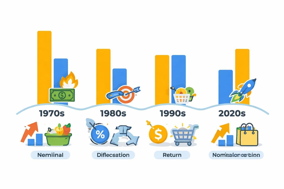
One of the most critical distinctions in historical market analysis involves separating nominal returns from real returns adjusted for inflation. The nominal rate of return shows the absolute percentage change in investment value, while the real return reflects purchasing power changes.
During the 1970s, many investments posted positive nominal returns but negative real returns as inflation rates exceeded investment gains. Conversely, the post-1982 period saw lower inflation rates enhance the real value of returns across most asset classes.
Calculating Inflation-Adjusted Returns
The real rate of return calculation subtracts the inflation rate from the nominal return:
Real Return ≈ Nominal Return - Inflation Rate
For more precise calculations, especially with higher inflation rates, the formula becomes:
Real Return = [(1 + Nominal Return) / (1 + Inflation Rate)] - 1
Understanding this distinction proves crucial when analyzing historical investment performance. A 15% nominal return during a period of 10% inflation delivers only a 4.5% real return, significantly impacting long-term wealth accumulation.
Time-Weighted Versus Money-Weighted Returns
Investment analysis often requires distinguishing between time-weighted and money-weighted return methodologies. Each approach serves different purposes and can produce different results for the same investment.
Time-weighted returns eliminate the impact of cash flow timing, measuring only the investment's performance. This method proves ideal for comparing fund managers or investment strategies since it removes the effect of investor contributions and withdrawals.
Money-weighted returns, conversely, incorporate the timing and size of cash flows, reflecting the actual investor experience. This approach matters more when evaluating personal investment outcomes, as it captures whether investors successfully timed their contributions.
| Return Type | Best Used For | Accounts for Cash Flow Timing | Typical Applications |
|---|---|---|---|
| Time-Weighted | Manager performance | No | Mutual fund comparisons, strategy evaluation |
| Money-Weighted | Investor experience | Yes | Personal portfolio returns, retirement account analysis |
| Simple | Single-period holdings | Not applicable | Individual stock trades, bond holdings |
| Annualized | Multi-year comparisons | No | Long-term performance benchmarking |
Historical market analysis benefits from understanding both methodologies. Studying how investors fared during market crashes often reveals that poor timing of contributions (money-weighted effects) exacerbated losses beyond what the market itself experienced (time-weighted performance).
Risk-Adjusted Return Metrics
Examining the rate of return without considering risk provides an incomplete picture of investment performance. Two investments might deliver identical 12% annual returns, but one might achieve this with far greater volatility than the other.
Sharpe Ratio and Historical Context
The Sharpe ratio divides excess return (return above the risk-free rate) by the investment's standard deviation, creating a risk-adjusted performance measure. Higher Sharpe ratios indicate better risk-adjusted returns.
Analyzing historical Sharpe ratios across different market periods reveals how risk-return tradeoffs evolve. The 1950s and 1960s generally offered favorable Sharpe ratios for equities, while the 1970s saw these ratios compress as volatility increased without commensurate return improvements.
Other Risk-Adjusted Measures
Several additional metrics help contextualize returns relative to risk:
- Sortino Ratio: Focuses only on downside volatility rather than total volatility
- Treynor Ratio: Uses beta (market sensitivity) instead of total volatility
- Calmar Ratio: Compares annualized return to maximum drawdown
- Information Ratio: Measures excess return per unit of tracking error
When exploring historical financial events, these risk-adjusted measures provide deeper insights than raw returns alone. The 1987 crash, for instance, temporarily devastated Sharpe ratios despite relatively quick market recovery.
Sector and Industry Return Patterns
Historical market data reveals distinct patterns in how different sectors and industries generate returns over time. Technology stocks, for example, have experienced boom-bust cycles with extraordinary gains followed by severe corrections.
The dot-com era of the late 1990s saw technology stocks deliver triple-digit annual returns before collapsing in 2000-2002. Meanwhile, defensive sectors like utilities and consumer staples typically produce more modest but stable returns across market cycles.
Cyclical Versus Defensive Sector Performance
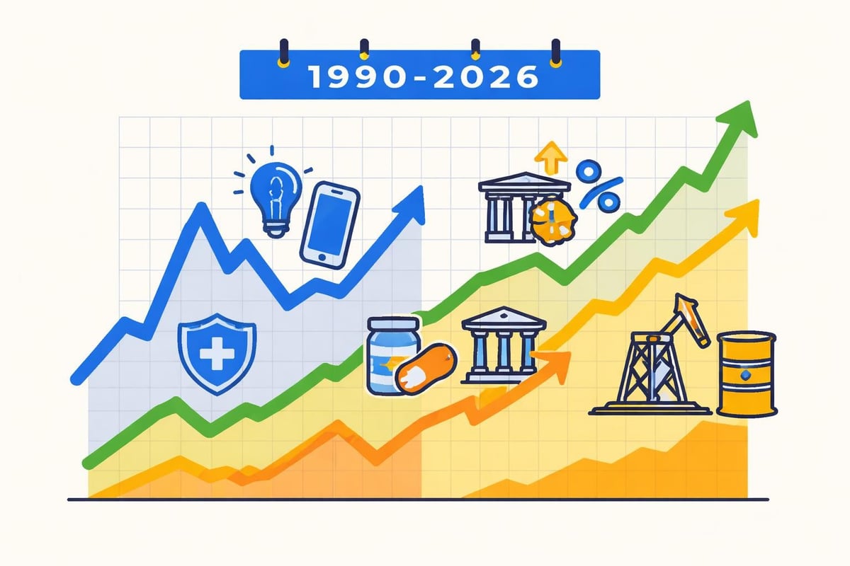
Understanding these patterns helps investors contextualize current market conditions within historical frameworks:
- Energy sectors tend to correlate with commodity price cycles and geopolitical events
- Financial stocks perform based on interest rate environments and credit conditions
- Consumer discretionary follows economic expansion and contraction patterns
- Healthcare and pharmaceuticals often show less correlation with economic cycles
- Industrial sectors closely track manufacturing and global trade activity
Studying how the operating margin and profitability metrics of these sectors evolved during past market environments provides valuable context for assessing current valuations and expected returns.
International and Emerging Market Returns
Geographic diversification introduces another dimension to rate of return analysis. Developed international markets have historically delivered returns comparable to U.S. markets but with different timing and volatility characteristics.
Emerging markets present a more complex picture. While offering potentially higher long-term returns, these markets also carry significantly greater volatility and political risk. The Asian financial crisis of 1997-1998 and the 2013 "taper tantrum" illustrate how emerging market returns can experience severe compression during stress periods.
Currency Impact on International Returns
International investments face currency risk that can substantially alter returns for U.S.-based investors. A European stock might rise 10% in euro terms, but if the euro depreciates 8% against the dollar, the U.S. investor's return falls to approximately 2%.
Historical analysis of international returns requires separating local currency returns from dollar-denominated returns. The period from 2002-2008 saw strong local currency returns in many markets enhanced by dollar weakness, while 2014-2016 experienced the opposite dynamic.
Fixed Income Return Characteristics
Bond returns follow different patterns than equity returns, with interest rate movements playing the dominant role. When rates fall, existing bonds with higher coupons increase in value, generating positive returns beyond the stated yield. Rising rates produce the opposite effect.
The great bond bull market from 1981-2020 saw interest rates decline from double digits to near zero, producing extraordinary returns for fixed income investors. Examining this period illustrates how floating rate instruments and fixed-rate bonds respond differently to rate changes.
Credit Quality and Return Spreads
Within fixed income markets, credit quality significantly impacts returns:
| Bond Category | Average Annual Return (1990-2025) | Default Rate | Return Volatility |
|---|---|---|---|
| Treasury Bonds | 5.2% | 0% | Low |
| Investment-Grade Corporate | 6.4% | 0.1% | Moderate |
| High-Yield Bonds | 8.7% | 3.8% | High |
| Emerging Market Debt | 9.3% | 5.2% | Very High |
Understanding these historical spreads helps investors assess whether current compensation for credit risk appears adequate relative to past periods. The 2008 financial crisis saw credit spreads widen dramatically as non-performing loans surged, creating both risks and opportunities.
Learning from Historical Return Patterns
Studying past market returns reveals several consistent patterns that inform investment decision-making. Mean reversion suggests that exceptionally high or low returns tend to move back toward historical averages over time. Markets that significantly outperform often experience subsequent periods of underperformance, and vice versa.
The concept of efficient market hypothesis suggests that consistently achieving above-market returns proves extremely difficult, as prices already reflect available information. Historical data supports this view for most active managers, with few consistently outperforming their benchmarks after fees.
Volatility and Return Relationships
Higher volatility typically accompanies higher long-term returns, compensating investors for accepting greater uncertainty. Small-cap stocks demonstrate this principle, delivering superior returns over long periods while experiencing sharper drawdowns during market stress.
The 2008 financial crisis exemplified this relationship, with high-volatility assets suffering the steepest declines before ultimately recovering to new highs. Investors who maintained exposure through the downturn eventually captured the recovery gains, while those who sold locked in losses and often missed the rebound.
Practical Applications for Modern Investors
Contemporary investors can apply historical rate of return analysis in several practical ways. First, understanding normal ranges of returns for different asset classes helps set realistic expectations and avoid chasing unsustainable performance.
Second, examining how different investments performed during specific historical events-recessions, inflationary periods, technological disruptions-provides context for current market conditions. While history doesn't repeat exactly, studying past patterns often identifies relevant parallels.
Third, evaluating investment proposals becomes more rigorous when compared against historical benchmarks. A strategy claiming to deliver consistent 15% annual returns with low volatility should be viewed skeptically given that such combinations rarely appear in historical data.
Building Historical Context into Investment Decisions
Investors benefit from asking several questions when evaluating opportunities:
- How does the promised return compare to historical averages for similar investments?
- What level of volatility has historically accompanied similar return profiles?
- During which historical periods would this strategy have struggled or excelled?
- How have regulatory changes or market structure evolution affected comparable investments?
- What role does capital expenditure play in sustaining competitive advantages and returns?
These questions help ground expectations in reality while identifying when opportunities might genuinely differ from historical patterns due to structural changes or unique circumstances.
The Role of Dividends and Income in Total Returns
Many investors underestimate how significantly dividends contribute to long-term equity returns. Historical analysis from established research sources shows that dividend income accounts for approximately 40% of total stock market returns over extended periods.
During the mid-20th century, dividend yields often exceeded bond yields, reflecting investors' preference for the perceived safety of fixed income. This relationship inverted during the 1980s and 1990s as investors increasingly valued growth over income.
Dividend Reinvestment Impact
Reinvesting dividends rather than taking them as cash dramatically enhances compound returns over time. An investment in the S&P 500 from 1990-2025 with dividends reinvested would have substantially outperformed the same investment without reinvestment.
This compounding effect proves particularly powerful during market downturns, as reinvested dividends purchase shares at depressed prices that subsequently recover. The 2008-2009 period demonstrated this dynamic, with reinvested dividends buying shares at crisis valuations that later appreciated significantly.
Mastering the rate of return concept and its historical patterns equips investors with essential tools for evaluating opportunities and understanding market behavior across different conditions. Whether analyzing individual securities, asset class performance, or overall portfolio results, this fundamental metric provides the foundation for informed decision-making. Historic Financial News helps investors deepen this understanding by providing interactive historical market data, AI-powered analysis of past market events, and contextual coverage that reveals the stories behind significant return patterns, empowering you to learn from history and make more informed investment decisions today.