J-Curve Guide: Insights, Effects, and Trends for 2026

Imagine steering your business or investment portfolio through the unpredictable global markets of 2026. Rapid technological change, shifting trade policies, and evolving consumer behavior demand a deeper understanding of economic cycles. One concept that stands out in this environment is the j-curve—a pattern that explains why initial setbacks often precede strong recoveries.

Today, the j-curve is more relevant than ever. It offers powerful insights for leaders, investors, and policymakers seeking to navigate periods of short-term decline and position for long-term growth.

This article serves as your comprehensive guide to the j-curve. You will discover its core definitions, explore real-world economic and financial applications, and follow the step-by-step evolution of j-curve effects across sectors. We will also examine future trends shaping the j-curve in 2026, equipping you with practical knowledge for the challenges and opportunities ahead.

Understanding the J-Curve: Definition and Core Concepts

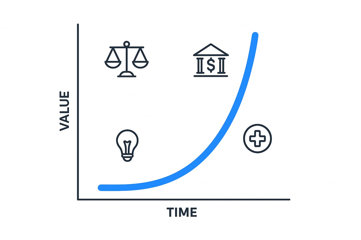
The j-curve is a powerful concept that helps explain why some economic or financial changes lead to an initial setback, followed by a substantial recovery. Its intuitive shape—a sharp dip that rebounds upward—makes it easy to visualize on a graph. By understanding the j-curve, analysts can better predict the stages of change in areas like trade, investment, and business cycles.

What is the J-Curve?

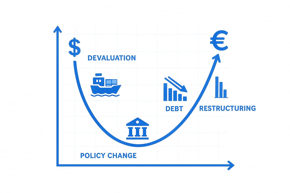
The j-curve describes a process where things get worse before they get better, forming a "J" shape when visualized. This term originally appeared in economics to illustrate how a country’s trade balance might deteriorate after currency devaluation, only to improve later as exports become more competitive.

It’s important to distinguish the j-curve from other patterns:

Curve Type	Shape	Typical Context
J-curve	Dip then rise	Trade, private equity
S-curve	Slow, rapid, then plateau	Innovation, adoption
L-curve	Sharp drop, slow recovery	Recessions, crises

For example, after a currency devaluation, imports may remain costly while export gains take time to materialize, resulting in a j-curve. This effect has been observed in real-world cases, such as U.S. trade data, as discussed in The J-curve revisited: an empirical examination for the United States.

Historical Context and Theoretical Foundations

The j-curve’s roots trace back to international trade theory, where economists like Stephen Magee and Robert Stern studied delayed positive outcomes after policy shifts. The concept gained traction during the 1970s and 1980s, particularly when analyzing trade balances and exchange rates.

Over time, the j-curve was adopted in fields beyond economics, such as private equity and even medicine. In these areas, the j-curve explains why returns or health outcomes may worsen before showing improvement. Major events—such as currency crises in Latin America or trade reforms in Asia—provided real-world evidence of the j-curve’s predictive value.

Key Variables and Determinants

Several factors determine the strength and timing of the j-curve effect. The elasticity of demand for imports and exports plays a central role. If consumers quickly switch to cheaper domestic goods after a currency devaluation, the j-curve recovery is faster.

Other key variables include:

• Competitiveness of local industries
• Policy environment (tariffs, subsidies)
• Time lags in trade contracts
• Global economic conditions and sentiment

Government actions can amplify or soften the j-curve. Historical data suggest that recovery periods may range from a few months to over a year, depending on these variables.

Types of J-Curve Effects

The j-curve appears in several contexts. In macroeconomics, it’s seen in trade balances after currency changes. In finance, private equity funds often show early losses before gains, mirroring the j-curve. Startups may also experience initial setbacks before rapid growth.

Other examples include:

• Public health, where interventions show delayed improvements
• Corporate restructuring, with short-term pain preceding long-term efficiency

The shape and length of the j-curve vary by situation, but understanding it is crucial for policymakers, investors, and business leaders as we approach 2026.

The J-Curve in Economics: Trade, Currency, and Policy Impacts

Understanding the j-curve effect is crucial for anyone navigating the complexities of global economics in 2026. The concept helps explain why economies often face initial setbacks before achieving lasting gains. Below, we explore its impact across trade, policy, and financial stability, providing real-world examples and critical analysis.

The J-Curve Effect in International Trade

The j-curve is most famously seen in international trade, particularly when a country devalues its currency. Initially, the trade balance often worsens, as import contracts remain costly and exports do not immediately pick up. Over time, however, exports become more competitive, and the trade balance improves, creating the signature "J" shape.

For example, after the UK’s Brexit vote and subsequent currency drop, its trade deficit widened before recovering. Similar patterns were observed during the Asian financial crisis and in several Latin American economies. Historical data shows that, on average, the positive phase of the j-curve may take 6 to 18 months to materialize.

Key factors influencing this timeline include the elasticity of demand for exports and imports, the speed of contract renegotiations, and global economic sentiment. In periods of stagflation, the expected j-curve recovery may be delayed or muted, as discussed in trade balance and economic cycles. Policymakers and investors must monitor these variables closely to anticipate the full impact.

Policy Shocks and Economic Reforms

Major policy changes can set off a j-curve effect across an entire economy. When governments introduce fiscal or monetary reforms, such as tax overhauls or deregulation, there is often an initial period of pain. GDP growth may slow, unemployment can rise, and confidence may falter.

Emerging markets provide clear examples. Structural reforms in countries like India and Brazil have triggered short-term slowdowns, followed by robust growth once new efficiencies and investments take hold. The j-curve dynamic is visible in the lag between policy implementation and economic rebound.

Public expectations and investor confidence are critical in shaping the curve’s trajectory. When stakeholders believe in the long-term benefits, the adjustment phase may be shorter, and recovery more pronounced. Statistics from previous reforms show that the inflection point often occurs within two to three years, but timing varies based on policy scope and market response.

The J-Curve in Sovereign Debt and Balance of Payments

The j-curve also plays a pivotal role in sovereign debt restructuring and balance of payments adjustments. Countries entering IMF programs or negotiating debt relief often face immediate hardships—budget cuts, austerity, and recession. In the short run, these measures deepen economic pain and can unsettle financial markets.

Case studies from Greece’s debt crisis and Argentina’s currency adjustments illustrate this effect. After initial contractions, both nations eventually stabilized, with credit ratings and bond yields improving over time. International investors watch these developments closely, as the j-curve shape helps forecast the transition from short-term losses to long-term gains.

For policymakers, understanding the j-curve is vital for planning recovery strategies and communicating realistic timelines to the public. It underscores the importance of resilience during the initial decline and strategic action to accelerate the upward phase.

Limitations and Critiques of the J-Curve in Economics

Despite its popularity, the j-curve is not a universal rule. In some cases, the expected recovery fails to materialize, especially when demand for exports is inelastic or structural weaknesses persist. Japan’s "lost decade" and chronic trade deficits in certain economies serve as cautionary tales.

Critics argue that the j-curve oversimplifies complex adjustment processes. Recovery often depends on complementary policies, such as education, infrastructure, or innovation incentives. Recent academic debates question the predictive power of the j-curve and emphasize the need for nuanced analysis.

For 2026, leaders must recognize both the potential and the limits of the j-curve. A clear-eyed approach, grounded in data and scenario planning, will help avoid pitfalls and maximize the benefits of economic transitions.

The J-Curve in Finance: Private Equity, Investments, and Business Growth

The j-curve is a defining feature in the world of finance, shaping how investors, fund managers, and business leaders approach risk, timing, and growth. Understanding its phases is crucial for anyone seeking to navigate private equity, venture capital, and the dynamic landscape of business expansion. Let’s explore how the j-curve manifests across financial domains and why its lessons are essential for success in 2026.

J-Curve Dynamics in Private Equity and Venture Capital

In private equity and venture capital, the j-curve describes the typical return pattern funds experience over time. Early in a fund’s lifecycle, negative returns are common. This is due to upfront management fees, investment costs, and the time required for portfolio companies to mature.

As investments progress, value creation accelerates. Exits and distributions begin to outpace costs, causing the j-curve to swing upward. Investors who recognize this pattern understand the importance of patience and a long-term outlook.

Industry benchmarks show that positive cumulative returns often emerge three to five years into a fund’s life. Real-world data indicates that the depth and duration of the j-curve can vary, influenced by market cycles and exit environments. For a deeper dive into these dynamics, see Risk and return in private equity, which explains how the j-curve affects investor outcomes and risk assessment.

The j-curve is not just a theoretical model. It shapes fund strategies, investor expectations, and performance measurement. Private equity professionals closely monitor this effect to optimize timing and maximize returns.

Applications in Corporate Strategy and Project Management

The j-curve effect is also evident in corporate strategy, especially during major transformations. When companies restructure, launch digital initiatives, or pursue mergers and acquisitions, initial performance often declines before improvements materialize.

Leaders face challenges such as cultural resistance, integration costs, and operational disruptions. The j-curve reminds executives to anticipate this early dip and communicate transparently with stakeholders.

• Common triggers for a corporate j-curve:
  • Large-scale IT upgrades
  • Organizational restructuring
  • Mergers and acquisitions
  • R&D investments

To accelerate the upward phase, companies use strategies like agile project management, phased rollouts, and continuous feedback loops. This approach helps shorten the adjustment period and capitalize on competitive advantages as momentum builds.

Understanding the j-curve enables decision-makers to align resources, manage expectations, and foster resilience during times of change.

J-Curve Patterns in Startup and Small Business Growth

Startups and small businesses frequently encounter the j-curve as they scale. Early-stage ventures often burn cash and report losses, reflecting the steep investment required for product development, market entry, and customer acquisition.

Once a startup achieves product-market fit and operational efficiencies, growth accelerates rapidly. This creates the upward swing of the j-curve, with revenues and profits rising faster than costs.

Several factors shape the j-curve’s depth and length in small businesses:

• Market demand and competition
• Access to funding
• Team experience
• Speed of innovation

Real-world examples include SaaS startups, which may take years to reach profitability, and fintech disruptors that endure early losses before capturing significant market share. Entrepreneurs and investors who understand the j-curve are better equipped to set realistic milestones and persevere through initial challenges.

Investment Strategies and Risk Management

Recognizing the j-curve is vital for constructing resilient investment portfolios. Investors must account for early-stage losses and delayed gains, especially in private equity, venture capital, and high-growth sectors.

Effective strategies include:

• Diversification across asset classes and vintage years
• Staggered capital commitments to balance cash flows
• Scenario analysis and stress testing to anticipate downturns

Advanced tools, such as real-time dashboards and benchmarking platforms, help track j-curve progress and inform tactical decisions. Historical fund performance studies reveal that portfolios prepared for the j-curve’s timing achieve superior risk-adjusted returns.

By embracing the j-curve framework, investors and business leaders can better manage volatility, align expectations, and position themselves for long-term growth in the evolving financial landscape.

Step-by-Step: How the J-Curve Effect Unfolds

Understanding how the j-curve unfolds step by step is essential for anyone navigating economic cycles or investment lifecycles. Each phase of the j-curve reveals unique challenges and opportunities, shaping decision-making and long-term outcomes.

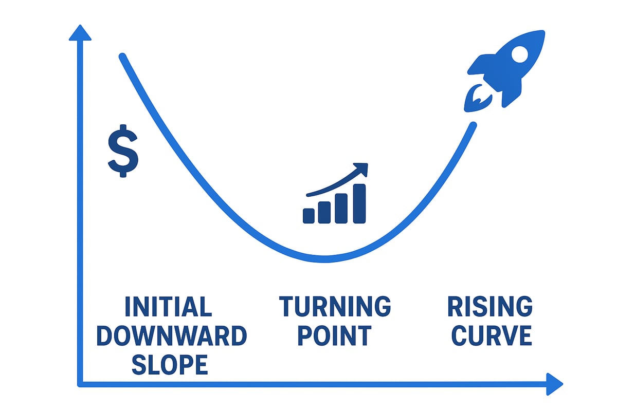
Phase 1: Initial Decline

The first phase of the j-curve is marked by an immediate downturn. This decline can result from adjustment costs, market inertia, or psychological factors like uncertainty. In economic contexts, negative returns, widening deficits, or declining sales often surface right after policy changes or investments.

For example, after a currency devaluation, a country may experience a worsening trade balance as import prices rise and export contracts remain fixed. In private equity, early fund performance can dip due to fees and startup costs. This mirrors what is observed in Private equity and J-curve returns, where initial losses precede later gains.

Resilience and clear communication are vital during this stage. Historical data shows that the depth of the initial decline varies by context, but enduring this phase is key to realizing future benefits.

Phase 2: Adjustment and Inflection Point

As the j-curve progresses, markets, consumers, and stakeholders begin to adapt. This adjustment phase is driven by factors such as increased price sensitivity, operational efficiencies, and competitive repositioning.

A classic example is when export demand rises as goods become more competitively priced after a currency adjustment. In business, companies may streamline operations or pivot strategies, leading to gradual stabilization.

Policy support and positive market signals are crucial in reaching the inflection point, where the downward trend halts and recovery begins. On average, this turnaround can occur several months after the initial shock, depending on the sector and external conditions.

Recognizing this phase helps decision makers anticipate the tipping point where losses start converting into gains.

Phase 3: Sustained Recovery and Growth

The third phase of the j-curve is characterized by a steady upward trajectory. Trade balances improve, investment returns rise, and confidence builds across markets. Compounding effects often accelerate progress, further reinforcing the recovery.

Case studies from post-crisis economies and successful fund exits highlight how the j-curve can lead to significant growth once the inflection point is surpassed. For instance, countries that implemented effective reforms often see robust gains after the initial pain.

Maximizing gains during this period involves capitalizing on momentum and maintaining strategic focus. Data shows that the magnitude and duration of recovery depend on both internal resilience and external opportunities.

Common Pitfalls and How to Avoid Them

Navigating the j-curve comes with risks. Common mistakes include underestimating time lags, overleveraging resources, and failing to communicate transparently. These errors can deepen losses or delay recovery.

To mitigate these risks, consider:

• Scenario planning to anticipate challenges
• Stress testing financial and operational plans
• Maintaining transparent reporting to stakeholders

Several failed recoveries stem from impatience or neglecting real-time data. Embracing patience and a long-term vision is essential for riding out the j-curve successfully.

Monitoring and Measuring the J-Curve Effect

Effective tracking is crucial for managing the j-curve. Key performance indicators (KPIs) vary by context but may include trade balances, return on investment, or sales growth.

Modern tools like dashboards and analytics platforms enable real-time monitoring. Benchmarking against historical j-curve patterns helps contextualize progress. Organizations increasingly use data-driven approaches to adapt strategies as new information emerges.

Regular measurement and adjustment provide the feedback needed to stay on course, ensuring that the j-curve delivers the expected outcomes.

Sector-Specific J-Curve Effects: Case Studies and Insights for 2026

The j-curve effect does not manifest uniformly across all industries. Understanding its sector-specific nuances helps leaders, investors, and policymakers anticipate both challenges and opportunities. By exploring how the j-curve unfolds in emerging markets, private equity, technology, public policy, and leadership strategies, we can draw actionable insights for 2026.

J-Curve in Emerging Markets and Global Trade

Emerging markets often experience pronounced j-curve effects following currency adjustments or economic reforms. For instance, after a devaluation, countries like Argentina or Nigeria initially see trade deficits widen as import costs surge. However, over the next 12–24 months, exports become more competitive, reversing the trend and driving a robust recovery.

Short-term pain is common, but the j-curve rewards patient investors who understand the timing. Supply chain shifts in Asia and Africa are prime examples, where reforms in 2024–2025 are expected to yield gains in 2026. Nevertheless, risks remain: sudden capital outflows or weak domestic demand can delay or distort the upward phase.

For global supply chains, recognizing the j-curve is critical. Firms able to anticipate and adapt to these cycles can secure first-mover advantages as new markets stabilize and grow.

Private Equity and Alternative Investments in 2026

In private equity, the j-curve describes the early years of negative or flat returns as funds deploy capital, pay fees, and restructure portfolio companies. Only as value creation and exits materialize do returns shift upward, often after year three or four.

Recent industry surveys forecast that the j-curve shape may steepen in 2026, given macroeconomic uncertainty and regulatory shifts. Investors should expect longer periods before distributions accelerate. To navigate this, experts recommend robust due diligence and patience, as highlighted in Mapping the venture capital and private equity research: a bibliometric review and future research agenda.

Alternative assets, such as infrastructure and real estate, also show j-curve dynamics, especially in emerging markets. Understanding these patterns helps investors balance portfolios and set realistic expectations.

Technology and Innovation-Driven Industries

Tech sectors like fintech, AI, and green energy frequently display j-curve growth trajectories. Startups in these spaces often incur heavy upfront R&D costs, with delayed profitability. However, once product-market fit is achieved, revenues and valuations can surge rapidly.

Data from global startup hubs shows time-to-profitability averages 2–5 years, with the j-curve especially visible in SaaS and platform-driven models. Growth stocks in these industries are a classic example, as explained in Growth stock investment dynamics, where initial volatility gives way to exponential gains.

For 2026, expect continued innovation-driven j-curve effects, especially as new technologies mature and adoption rates climb. Strategic patience and targeted investment are essential to harness these opportunities.

Public Policy, Health, and Social Change

The j-curve is not limited to finance or trade; it also appears in public policy and health interventions. Consider vaccination campaigns—initial rollout costs and disruptions may precede measurable public health improvements. Similarly, education reforms or universal basic income pilots often encounter skepticism and short-term setbacks before benefits become evident.

During pandemic recovery efforts, countries implementing swift but disruptive measures saw economic and social indicators dip before rebounding stronger. The j-curve here highlights the importance of stakeholder engagement and transparent communication.

Policymakers must recognize that delayed payoffs are typical. Building public trust and maintaining momentum through the trough of the j-curve can determine long-term success.

Lessons for Leaders and Decision Makers

For executives, investors, and policymakers, mastering the j-curve is essential for effective strategy. Scenario planning and adaptive leadership are vital when navigating the initial downturns and positioning for recovery.

Key lessons include managing expectations, prioritizing clear communication, and leveraging data-driven frameworks to monitor progress. Balancing short-term pain with long-term vision helps organizations avoid common pitfalls.

Ultimately, the j-curve teaches that resilience, foresight, and agility are crucial traits for success in 2026’s fast-evolving global landscape. Leaders who understand and act on j-curve dynamics can turn periods of adversity into platforms for growth.

Future Trends: The Evolving J-Curve Landscape for 2026

Navigating the future means staying ahead of the rapid shifts shaping the global economy. The j-curve, once a traditional economic concept, is now central to forecasting market cycles, investment outcomes, and policy impacts in 2026. As new forces reshape industries, understanding j-curve dynamics will be key for anyone aiming to thrive amid uncertainty.

Macroeconomic Outlook and J-Curve Projections

In 2026, the j-curve is expected to play a critical role in global economic forecasts. Currency fluctuations, trade reforms, and policy shifts will likely trigger pronounced j-curve patterns, especially in emerging markets. According to projections from the IMF and World Bank, several regions will experience initial downturns following policy changes, with recoveries anticipated as markets adapt.

A quick comparison of anticipated j-curve impacts:

Region	Trigger Event	Initial Decline	Recovery Timeline
Asia	Trade Liberalization	6 months	12-18 months
Latin America	Currency Devaluation	9 months	18-24 months
Europe	Fiscal Reforms	3 months	9-15 months

Geopolitical tensions and supply chain disruptions may add volatility, yet proactive adaptation can help smooth the j-curve’s trajectory. For investors, understanding risk-adjusted investment performance is crucial when positioning portfolios during the early phases of the j-curve, as it helps balance short-term setbacks with long-term growth.

Technological Advancements and Data Analytics

Technology is revolutionizing j-curve analysis. AI, big data, and advanced predictive analytics now allow organizations to monitor and forecast the j-curve in real time. These tools help identify inflection points earlier, empowering investors and policymakers to act decisively.

A notable development is the application of supervised neural networks for forecasting cash flows in illiquid assets, such as private equity funds that often follow a j-curve pattern. For a deeper dive into these predictive modeling techniques, see Supervised Neural Networks for Illiquid Alternative Asset Cash Flow Forecasting.

The adoption of digital dashboards and automated reporting streamlines j-curve tracking. As these capabilities expand, financial professionals can expect more precise scenario planning and risk assessment by 2026.

Sustainability, ESG, and the J-Curve

Sustainability and ESG trends are increasingly intersecting with the j-curve effect. Investments in green energy, social impact initiatives, and responsible governance frequently display j-curve-like adoption curves, where initial costs are followed by substantial long-term gains.

Recent data shows ESG funds experiencing early underperformance before strong rebounds, highlighting the importance of patience and strategic allocation. Regulatory support and shifting market preferences will likely amplify these effects in 2026. For investors, evaluating risk-weighted assets can provide a clearer picture of potential outcomes when navigating ESG-driven j-curve cycles. Integrating ESG metrics into j-curve analysis will be a growing priority for forward-thinking organizations.

Navigating Uncertainty: Strategies for 2026 and Beyond

Managing volatility during j-curve cycles requires robust strategies. Scenario planning, dynamic risk management, and agile decision-making will be essential for success. Organizations are advised to:

• Implement real-time data monitoring
• Develop contingency plans for different j-curve scenarios
• Foster adaptive leadership and transparent communication

By learning from best practices and industry leaders, firms can better weather the initial declines and position themselves for accelerated recovery. Continuous learning and flexibility are vital in harnessing the full potential of the j-curve in uncertain environments.

Emerging Research and Thought Leadership

Academic research on the j-curve is expanding rapidly. New theories explore its applications across finance, technology, health, and policy. Leading conferences, journals, and knowledge hubs are sharing insights on how to refine j-curve forecasting and management.

Experts emphasize the value of cross-disciplinary approaches, encouraging deeper collaboration between economists, data scientists, and industry practitioners. Readers are encouraged to stay engaged with emerging thought leadership to anticipate shifts in the j-curve landscape and drive innovation in their fields.

As we’ve explored, understanding the J curve can truly change the way you interpret financial markets and prepare for what’s next. Whether you’re an investor, a student, or just curious about market dynamics, having the right historical context is key to spotting real opportunities and avoiding common pitfalls. If you’re ready to get a deeper, interactive experience—where AI powered insights and historical data come together—why not be among the first to shape this new platform with us? Join Our Beta and help bring financial history to life for 2026 and beyond.